Lab 3: Introduction to R

Outline

Objectives

In this lab, you will learn

how to use RStudio
how to make a plot with R
how to do math in R, create objects, use functions, etc.,
ins and outs of a typical workflow in R

R Packages

No additional packages required this week.

Data

house prices
county elections

Grade

For this assignment, the only thing you will turn in on Canvas is a brief write up detailed at the end of the assignment. You will use R to create some statistics based on a new dataset.

Working in RStudio

Labeled Panes of RStudio

If you are going to do anything with R, RStudio is hands-down the best place to do it. RStudio is an open-source integrated development environment (or IDE) that makes programming in R simpler, more efficient, and most importantly, more reproducible. Some of its more user-friendly features are syntax highlighting (it displays code in different colors depending on what it is or does, which makes it easier for you to navigate the code that you’ve written), code completion (it will try to guess what code you are attempting to write and write it for you), and keyboard shortcuts for the more repetitive tasks.

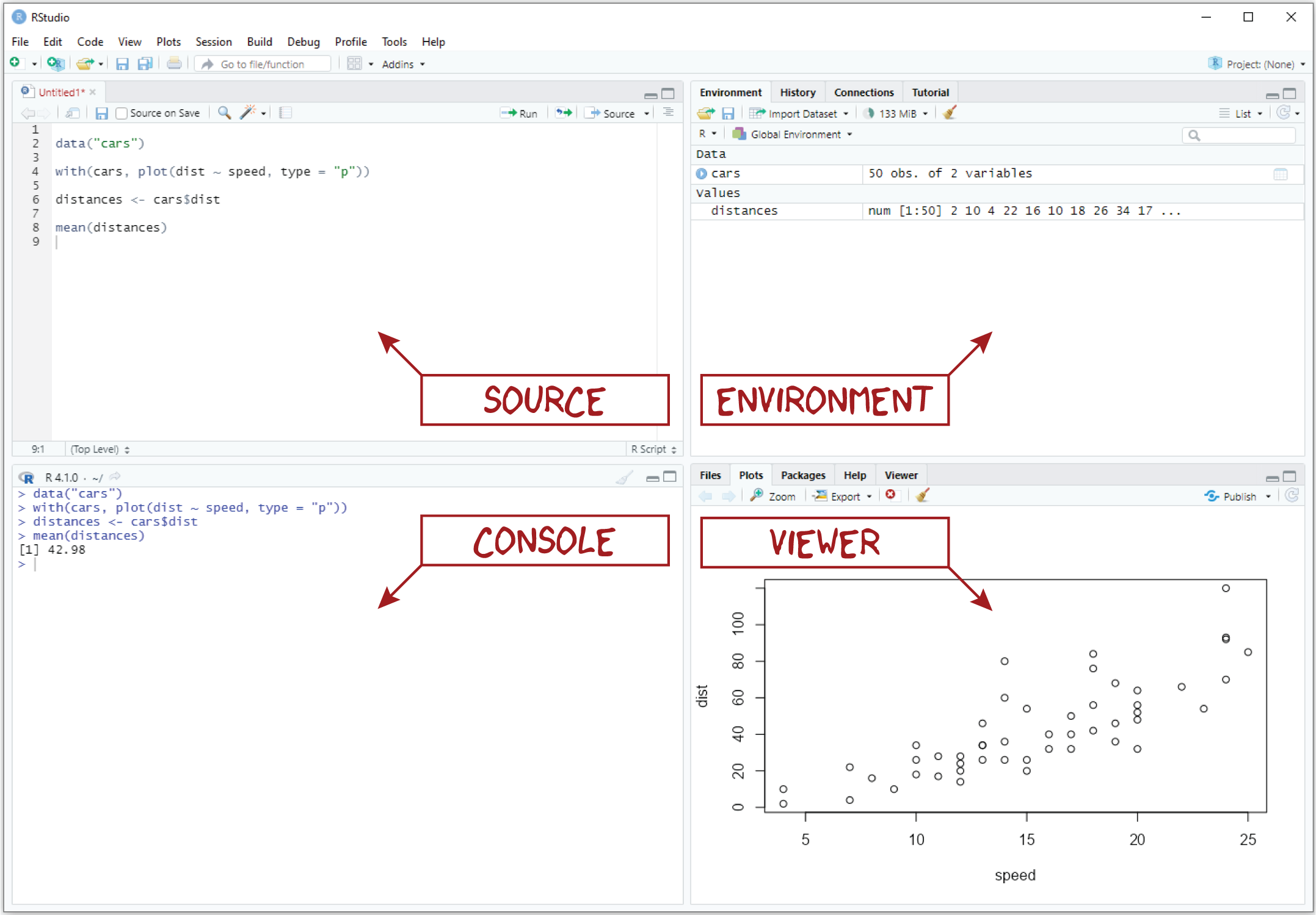
Pane layout

When you first open RStudio, you should see three window panes: the Console, the Environment, and the Viewer. If you open an R script, a fourth Source pane will also open. The default layout of these panes is shown in the figure above.

Source. The Source pane provides basic text editing functionality, allowing you to create and edit R scripts. Importantly, you cannot execute the code in these scripts directly, but you can save the scripts that you write as simple text files. A dead give away that you have an R script living on your computer is the .R extension, for example, my_script.R.
Console. The Console pane, as its name suggests, provides an interface to the R console, which is where your code actually gets run. While you can type R code directly into the console, you can’t save the R code you write there into an R script like you can with the Source editor. That means you should reserve the console for non-essential tasks, meaning tasks that are not required to replicate your results.
Environment. The Environment pane is sort of like a census of your digital zoo, providing a list of its denizens, i.e., the objects that you have created during your session. This pane also has the History tab, which shows the R code you have sent to the console in the order that you sent it.
Viewer. The Viewer pane is a bit of a catch-all, including a Files tab, a Plots tab, a Help tab, and a Viewer tab.
- The Files tab works like a file explorer. You can use it to navigate through folders and directories. By default, it is set to your working directory.
- The Plots tab displays any figures you make with R.
- The Help tab is where you can go to find helpful R documentation, including function pages and vignettes.

Let’s try out a few bits of code just to give you a sense of the difference between Source and Console.

As you work through this lab, you can practice running code in the Console, but make sure to do the actual exercises in an R script.

Exercises

First, let’s open a new R script. To open an R script in RStudio, just click File > New File > R Script (or hit Ctrl + Shift + N, Cmd + Shift + N on Mac OS).
Copy this code into the console and hit Enter.

rep("Boba Fett", 5)

Now, copy that code into the R script you just opened and hit Enter again. As you see, the code does not run. Instead, the cursor moves down to the next line. To actually run the code, put the cursor back on the line with the code, and hit Ctrl + Enter (CMD + Enter on Mac OS).

Setting up your R script

Working from an R script rather than the console is often preferred for several key reasons:

Reproducibility: An R script allows you to save all the code you write. This means you can easily rerun analyses, share your work, or troubleshoot without retyping commands. The console doesn’t keep a persistent record of the work unless you manually save it.
Efficiency: You can run large chunks of code or the entire script at once from an R script. In contrast, the console requires you to run each command one by one, which can slow you down, especially when working on complex analyses.
Error Tracking and Debugging: R scripts make it easier to track where things go wrong. You can add comments and sections, making the code easier to read and understand. If something fails, you can simply tweak a few lines and rerun without needing to rewrite everything.
Version Control: Scripts can be saved with comments about changes, making it easier to keep track of different versions of an analysis. The console provides no such history, meaning it’s harder to track revisions or recover earlier work.
Documentation and Collaboration: Writing code in an R script allows you to add detailed comments to explain your reasoning and the steps involved. This is especially useful when collaborating with others or when you return to a project after some time.
Organization: An R script enables you to organize your code logically, group tasks together, and maintain an overview of the entire workflow. The console can feel disorganized with scattered commands and no easy way to structure the work.

For students, especially those learning R, it’s a good habit to get comfortable with scripts early on. When you start a new assignment or project, you should create a header that includes a description of the code in the comments. To create comments (lines in the code that do not run), use the pound sign (#).

#### Lab 3: Introduction to R ####
# This code will use some basic functions in R and create a plot

R Basics

R is a calculator

You can just do math with it:

300 * (2/25)

[1] 24

3^2 + 42

[1] 51

sin(17)

[1] -0.9613975

Objects and Functions

But, R is more than just a calculator. There are a lot of things you can make with R, and a lot of things you can do with it. The things that you make are called objects, and the things that you do with objects are called functions. Any complex statistical operation you want to conduct in R will almost certainly involve the use of one or more functions.

Calling functions

To use a function, we call it like this:

function_name(arg1 = value1, arg2 = value2, ...)

Try calling the seq() function.

seq(from = 1, to = 5)

[1] 1 2 3 4 5

As you can see, this generates a sequence of numbers starting at 1 and ending at 5. There are two things to note about this. First, we do not have to specify the arguments explicitly, but they must be in the correct order:

seq(1, 5)

[1] 1 2 3 4 5

seq(5, 1)

[1] 5 4 3 2 1

Second, the seq() function has additional arguments you can specify, like by and length. While we do not have to specify these because they have default values, you can change one or the other (but not at the same time!):

seq(1, 10, by = 2)

[1] 1 3 5 7 9

seq(1, 10, length = 3)

[1]  1.0  5.5 10.0

Creating objects

To make an object in R, you use the arrow, <-, like so:

object_name <- value

Try creating an object with value 5.137 and assigning it to the name bob, like this:

bob <- 5.137

There are three things to note here. First, names in R must start with a letter and can only contain letters, numbers, underscores, and periods.

# Good
winter_solder <- "Buckey"
object4 <- 23.2

# Bad
winter soldier <- "Buckey" # spaces not allowed
4object <- 23.2            # cannot start with a number

Second, when you create an object with <-, it ends up in your workspace or environment (you can see it in the RStudio environment pane). Finally, it is worth noting that the advantage of creating objects is that we can take the output of one function and pass it to another.

x <- seq(1, 5, length = 3)

logx <- log(x)

exp(logx)

[1] 1 3 5

Exercises

Use seq() to generate a sequence of numbers from 3 to 12.
Use seq() to generate a sequence of numbers from 3 to 12 with length 25.
Why doesn’t this code work?

seq(1, 5, by = 2, length = 10)

Use <- to create an object with value 25 and assign it to a name of your choice.
Now try to create another object with a different value and name.
What is wrong with this code?

2bob <- 10

Analyzing Data

Load in some data

We will load in the data “house_prices.csv”, which is posted on Canvas. Save the data into a folder, preferably the same folder as where you are saving your R-script.

Set the working directory

You need to tell R what file folder you will be working out of. You can do this in two ways: 1. Go to the “Files” tab in the Viewer pane. Navigate to your folder, then hit the “More” icon, then select “Set As Working Directory”. Since you will want anybody who runs your code to set their working directory, copy the code from the console into your

2. Type the following code, but instead of your_file_path type the actual folder. Make sure your slashes are forward slashes ( / ) and not back slashes ( \ ).

setwd("your_file_path")

For example, in my script I will type the following, since that’s the folder I’m keeping my data in.

setwd("G:/My Drive/Classes/Regression Analysis")

Load in the data

Now that R knows where we have the data stored, we can load the data in.

house <- read.csv("data/house_prices.csv")

Note that I have my data in a subfolder of my working directory called “data”. Your code may look more like this:

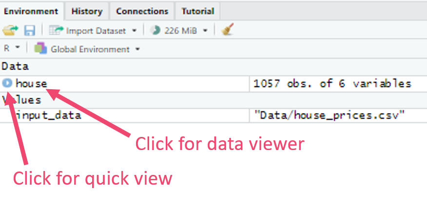
house <- read.csv("house_prices.csv")

This tells R to read in the csv and call the data frame “house”. You should see the data pop up in your environment. You can click on the word “house” and it will open up the data in the data viewer for you to explore. Or, if you just want a quick look, you can hit the little blue circle with the arrow next to the word “house”.

data viewing in the environment pane

We can also ask R to print the first few lines of a dataframe to show us what it looks like. In this case, each row represents a house.

head(house, n = 5) # The 5 tells R to print 5 rows

   Price Living.Area Bathrooms Age Fireplace Bedrooms
1 142212        1982         1 133         0        3
2 134865        1676         2  14         1        3
3 118007        1694         2  15         1        3
4 138297        1800         1  49         1        2
5 129470        2088         1  29         1        3

The Price is how much the house sold for. The Living.Area is the number of square feet the house had. We also have the number of Bathrooms and Bedrooms. Finally, we have the Age of the house and whether it has a Fireplace.

Create some descriptive statistics

R can work as a calculator. Let’s try a few simple exercises. What is the mean and standard deviation of house price? Note that we have to tell R what data frame we’re getting the variable from (in this case “house”), then put a $ to let R know we’re retrieving an element of the data frame (in this case “Price”).

mean(house$Price)

[1] 167901.9

sd(house$Price)

[1] 77158.35

Make Your First Plot!

To ease you into working with R, let’s visualize some data to answer a simple question: Is the price of a house related to its square footage? Don’t worry about understanding every bit of code! It’s just to give you a feel for the sort of graphics you can make with R. We’ll spend a future lab learning how to make even better graphics.

The `plot()` function

The base R graphics package provides a generic function for plotting, which - as you might have guessed - is called plot(). (“Base R” means it’s automatically loaded and you don’t have to install it.) To see how it works, try running this code:

plot(house$Living.Area, house$Price)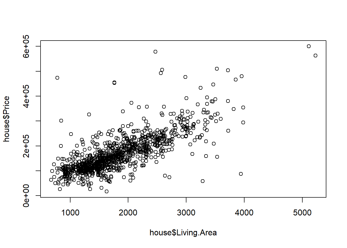

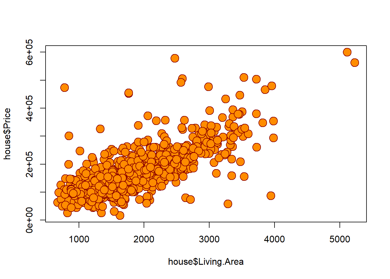
Customizing your plot

With the plot() function, you can do a lot of customization to the resulting graphic. For instance, you can modify all of the following:

pch will change the point type,
main will change the main plot title,
xlab and ylab will change the x and y axis labels,
cex will change the size of shapes within the plot region,
pch will change the type of point used (you can use triangles, squares, or diamonds, among others),
col changes the color of the point (or its border), and
bg changes the color of the point fill (depending on the type of point it is)

For instance, try running this code:

plot(
  house$Living.Area,
  house$Price,
  pch = 21,
  bg = "darkorange",
  col = "darkred",
  cex = 2
)

Exercises

Complete the following line of code to preview only the first three rows of the house table.

head(house, n = )

Modify the code below to change the size (cex) of the points from 2 to 1.5.

plot(
  house$Living.Area,
  house$Price,
  pch = 21,
  bg = "darkorange",
  col = "darkred",
  cex = 2
)

What does this plot tell us about the relationship between house size and price? Is it positive or negative? Or is there no relationship at all? If there is a relationship, what might explain it?
Complete the code below to add “Scatter Plot of House Size and Price” as the main title.

plot(
  house$Living.Area,
  house$Price,
  pch = 21,
  bg = "darkorange",
  col = "darkred",
  cex = 1,
  main = 
)

Complete the code below to add “House size (sq. ft.)” as the x-axis label and “Price ($)” as the y-axis label.

plot(
  house$Living.Area,
  house$Price,
  pch = 21,
  bg = "darkorange",
  col = "darkred",
  cex = 2,
  main = "Scatter Plot of House Size and Price",
  xlab = ,
  ylab = 
)

Assignment

Now it’s time to work on your own. Download the “County_Election.csv” data set from Canvas and put it in your working directory. Read in the data using read.csv(). Then, write a paragraph giving some information on the data that you find interesting. Include at least 3 statistics and one graph. Be sure to interpret what you think the significance of the statistic is.

Here is a table describing the variables in the data set:

Name	Description
state	State FIPS Code
county	County FIPS Code
county_name	County Name
state_name	State Name
fips	Combined FIPS Code
pct_republican_2016	Percent of voters in county that voted Republican in 2016 presidential election
frac_coll_plus2010	Percent of adults 25 years or older who have a 4-year college degree or more in 2010
foreign_share2010	Number of foreign born residents in the 2010 Census divided by the sum of native and foreign born residents.
med_hhinc2016	Median household income in 2016
poor_share2010	Share of families with incomes under the poverty line in 2010
share_black2010	Share of people who are Black in 2010
share_hisp2010	Share of people who are Hispanic in 2010
share_asian2010	Share of people who are Asian in 2010
rent_twobed2015	The median gross rent for renter-occupied housing units with two
popdensity2010	Number of residents per square mile in 2010
ann_avg_job_growth_2004_2013	Average annualized job growth rate over the time period 2004 to 2013

You may want to do different statistics from what we did above. Here are some functions you can use. To get information about them, type a question mark followed by the function you are looking up into the console. Alternatively, look the function up online.

Statistics

Statistic	Function
Minimum:	`min()`
Maximum:	`max()`
Average:	`mean()`
Standard Deviation:	`sd()`
Median:	`median()`
Percentiles:	`quantile()`
Correlation Coefficient:	`cor()`
Frequency tables:	`table()`
Relative Frequency tables:	`prop.table()`

Note that in frequency tables you can use more than one variable!

Graphics

Plot	Function
Bar chart:	`barplot()`
Histogram:	`hist()`
Box plots:	`boxplot()`
Scatter plot:	`plot()`

Outline

Objectives

R Packages

Data

Grade

Working in RStudio

Pane layout

Exercises

Setting up your R script

R Basics

R is a calculator

Objects and Functions

Calling functions

Creating objects

Exercises

Analyzing Data

Load in some data

Set the working directory

Load in the data

Create some descriptive statistics

Make Your First Plot!

The plot() function

Customizing your plot

Exercises

Assignment

Statistics

Graphics

The `plot()` function