Lecture 5: dplyr for Data Wrangling

This lecture introduces the core tools for data wrangling in R using the dplyr package. We will work with American Community Survey (ACS) microdata, which contains individual- or household-level observations rather than county-level averages.

ACS microdata allows us to ask richer economic questions, such as:

How do wages differ between citizens and non-citizens?
How does labor force participation vary by education?
How do outcomes differ across states or metro areas?

Because microdata is large and detailed, clean data workflows matter. The tools in this lecture are essential for preparing data for analysis and regression.

The Tidy Data Idea

Before learning functions, we need a clear data structure.

A dataset is tidy if:

Each row is one observation (one person or household)
Each column is one variable (wages, citizenship, education)
Each cell contains exactly one value

ACS microdata is usually close to tidy, but we often need to:

Select relevant variables
Recode or create new variables
Collapse individual data into group-level summaries

Loading Packages

library(dplyr)
library(ggplot2)

Load in the microdata csv:

acs <- read.csv("acs_microdata.csv")

Each row represents one person. The variables include:

AGE
SEX
CITIZEN (citizenship status)
INCTOT (total income)
EDUC (education category)
EMPSTAT (employment status)

Selecting Variables with `select()`

ACS files are large. The first step is usually to keep only what you need. We will remove the SEX variable for this analysis.

acs_small <- acs |>
  select(AGE, CITIZEN, INCTOT, EDUC, EMPSTAT)

This does not change the data—it creates a new dataset with fewer columns.

Filtering Observations with `filter()`

We often want to focus on a relevant population.

Example: Keep working-age adults with positive wage income.

acs_workers <- acs_small |>
  filter(AGE >= 25, AGE <= 64, INCTOT > 0)

Filtering rows is one of the most common steps in applied microdata analysis.

How many observations are left in the dataset? How many variables?

Creating New Variables with `mutate()`

ACS variables are often coded numerically. We frequently create indicators or transformed variables.

Example: Create a citizen indicator.

acs_workers <- acs_workers |>
  mutate(citizen_indicator = ifelse(CITIZEN == 3, 0, 1))

Example: Log wages (common in regression analysis) and create labor force indicators.

acs_workers <- acs_workers |>
  mutate(log_income = log(INCTOT),
         lab_force = ifelse(EMPSTAT %in% c(1,2), 1, 0))

We can use these new variables to compare groups using ggplot:

ggplot(data = acs_workers, aes(x = log_income,  fill = as.factor(citizen_indicator))) +
  geom_density(alpha = 0.5) +
  xlab("log(Total Income)") +
  labs(fill = "Citizen") +
  theme_classic()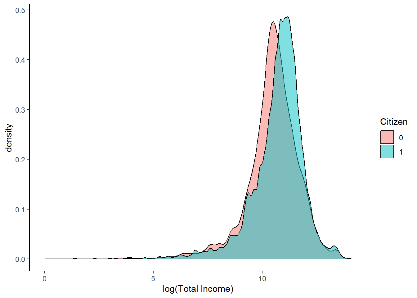

Grouped Summaries with `group_by()` and `summarize()`

Microdata becomes most powerful when we collapse it into meaningful groups.

Example: Average wages by citizenship status.

acs_workers |> 
  group_by(citizen_indicator) |> 
  summarize(
    avg_income = mean(INCTOT),
    num_obs = n()
  )

# A tibble: 2 × 3
  citizen_indicator avg_income num_obs
              <dbl>      <dbl>   <int>
1                 0     63503.    5552
2                 1     75679.   70269

This turns individual-level data into a group-level dataset.

A Complete Workflow Example

We can string together a number of dplyr functions in the order we want them done.

acs_summary <- acs |> 
  select(AGE, SEX, INCTOT, EDUC) |> # Select relevant rows
  filter(AGE >= 25, AGE <= 64, INCTOT > 0) |> # Filter out non-working age & missing income
  mutate(less_than_hs = ifelse(EDUC < 6, 1, 0)) |> # Create hs indicator
  group_by(less_than_hs, SEX) |> # Group by sex and hs indicator
  summarize(avg_income = mean(INCTOT)) # Find average income by group

This pipeline:

Chooses relevant variables
Filters the population
Creates a clean indicator
Produces a dataset ready for plotting or regression

Why This Matters for Economics

Most economic analysis is not about running regressions—it is about constructing the right dataset.

Using ACS microdata with dplyr allows you to:

Define populations precisely
Create economically meaningful variables
Aggregate data transparently
Avoid mistakes hidden by spreadsheet workflows

These skills are foundational for empirical work in labor, public, and applied microeconomics.

Exercise

Using ACS microdata:

Select age, citizenship, employment status, education, and wage variables
Keep individuals ages 25–64
Create a binary variable for non-citizens & for labor force status (EMPSTAT = 3 means the worker is not in the labor force)
Compute labor force participation by citizenship and education

Be prepared to explain each step of your pipeline in words.

The Tidy Data Idea

Loading Packages

Selecting Variables with select()

Filtering Observations with filter()

Creating New Variables with mutate()

Grouped Summaries with group_by() and summarize()